
This post will explain lossy compression algorithms, including Run Length Encoding, Dictionary coding, and the Huffman coding method typically discussed in the GCSE and A-Level syllabus (particularly OCR). Let’s recap the two different types of compression when it comes to data storage:
Lossy Compression
When data that is not important to the file is removed. Audio, Images, and Videos are good when used with lossy compression algorithms. MP3s are an example of this where sound quality may reduce but not to a point that is noticeable by the listener. JPEG is another example, where pixels are removed and combined so as to only appear as slight variations of colour in the image hardly noticeable to the human eye.
Lossless Compression
This is when data is temporarily removed from the file, but added back (rebuilt) when the file is to be used again. Zip files are an example of this. They will need to be unzipped (extracted) to be useable again.
Checkout my TES Shop for premium resources

Run Length Encoding
A simple form of lossless compression is called the Run Length Encoding algorithm. It shows the nature of lossless compression and how it seeks to find patterns of data that can be reconstructed later.
Consider the following attempt at a 1-bit image of a smiley:
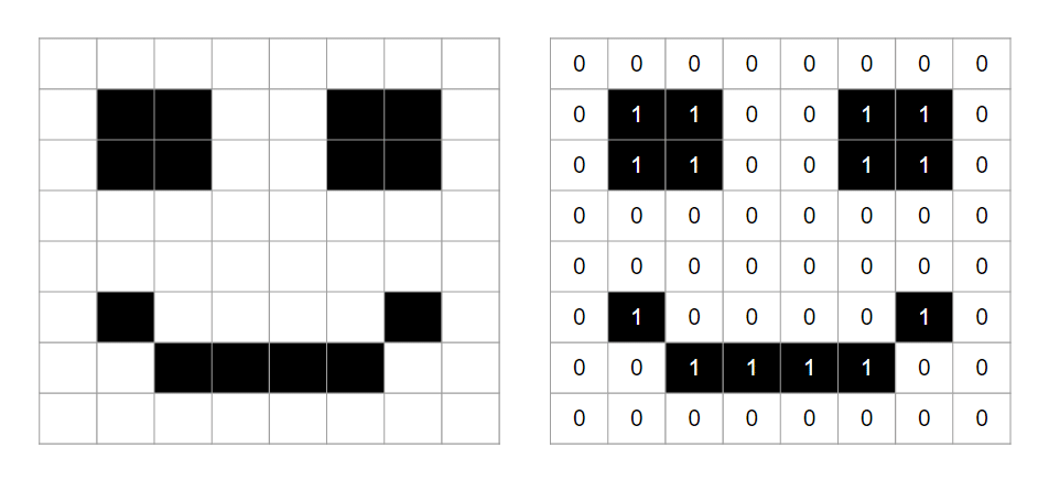
If we take the 1st row, for example, the data would ordinarily be 7 bits in length – 0000000.
However, run-length encoding would focus on the pattern of 5 white pixels in a row and so would store the data (whilst the file is compressed) as 7W or 101 0, which uses 1 fewer bit.
This is the main idea of Run Length Encoding. As images increase in size, there are a lot more similar shades that can be combined like this, reducing the file size by quite a lot. It is simple but effective.
Dictionary Coding
Another form of lossless comp[session. this method replaces the data in a file with “references” to what the data is. In the image, we have a dictionary with all of the words of the English language in. If we assign each a binary value we can then run through the data, replacing the words with the binary value/reference, thereby saving space as the binary value would more often than not be smaller than the space it would take to save the actual word. Let’s take a look using the example “I love Computer Science”
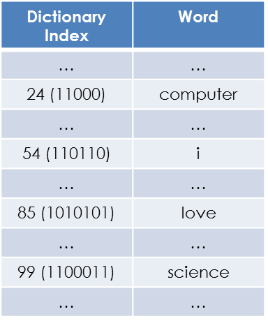
in this example, we can take each word and replace it with its binary reference.
11000 110110 1010101 1100011 which is just 25 bits.
This is smaller than storing each word. Even the word “computer” would require 64 bits if it was uncompressed.
The only downside would be that the size of the dictionary could be very large. This should not matter too much if the file size is large overall, however.
Huffman Coding
This is the more difficult of the three encoding methods. It uses a binary tree, which might seem complicated but it’s just a way for our computers to store information in an organised manner.
In each tree, we have nodes – which is equal to a piece of data. Each node will have a memory location and if it has children will point to other locations in memory. Each node will be pointing towards another piece of memory and may not be “next” to it in memory but it will be in a specific order.
Let’s look at how this algorithm is applied.
Suppose you have the statement “res rows”
With no compression it will have 64 bits as 8 * 8 bits = 64
- r = 01110010
- e = 01100101
- d= 01100100
- space = 00100000
- r = 01110010
- o = 01101111
- w = 01110111
- s = 01110011
| Character | Frequency |
| r | 2 |
| s | 2 |
| w | 1 |
| o | 1 |
| e | 1 |
| Space | 1 |
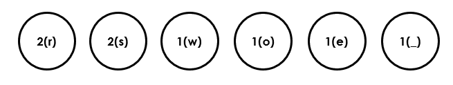
With Huffman Coding, we begin by counting the frequency of each character and adding it to a table.
Each character is then added to a node of a tree, starting with the most frequent character:
The Algorithm
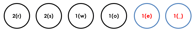
There are 3 main steps involved in this process. We repeat until all of our data has been converted into a binary tree then we can work out the binary value for the statement. Here are the steps:
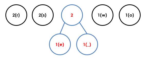
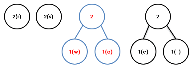
- Join (as a tree) the first two nodes from the right, adding the frequencies together and adding this sum to the root node.
- Re-insert the root node of the tree into the correct numerical position
- Repeat until only one node is left
Let’s now use diagrams to illustrate each step for the statement “red dogs”
Step 1
Step 2

Step 3
Step 4
Step 5

Step 6

Step 7
Step 8

Step 9

Step 10

Step 11
Step 12
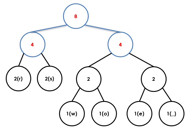
Now we add binary values to each branch using the following rule:
Left Branch = 0 & Right Branch = 1

Now just read from the top node down to create a binary bit string from the letters
r e s r o w s
r = 00 e = 110 s = 01 space = 111 r = 00 o = 101 w = 100 s = 01
That’s all for now, this should assist you in your GCSE Computer Science course if the requirements are to understand certain compression algorithms